DDPM
DDPM
OUTLINE
- Overall
- Forward Process (Diffusion Process)
- Reverse Process (Denoise)
- Optimization
- Trainning and Sampling
Overall
A Diffusion Model, specifically Deep Diffusion Probabilistic Models (DDPM), is a type of generative model that employs a diffusion process to generate data samples.
Here’s a brief explanation of DDPM:
Diffusion Process: DDPM uses a diffusion process where, initially, generated samples start as noisy versions, typically random. Over multiple steps, the strength of the noise is gradually reduced, making the samples closer to real data. Each step is modeled as a probability distribution, with parameters controlled by neural networks.
Deep Neural Networks: DDPM employs deep neural networks to model the probability distribution at each diffusion step. This allows it to learn complex data distributions and progressively reduce noise to make samples resemble training data.
Reverse Process: DDPM can be used not only for sample generation but also for estimating the probability density function of data. This makes it suitable for density estimation and sampling tasks like image generation, denoising, and super-resolution.
Training: Training DDPM involves estimating the parameters of probability distributions during the diffusion process to closely match the true distribution of the training data. Common training techniques include maximum likelihood estimation.
One significant advantage of DDPM is its ability to generate high-quality images and perform denoising tasks effectively. By iteratively improving sample quality, it can produce very realistic samples, particularly in the realm of image generation. However, compared to other generative models, DDPM’s training and generation processes can be more complex and time-consuming.
– Generated by ChatGPT 3.5
Forward Process (Diffusion Process)
The forward process is a markov chain containing discrete states from time step 0 to T. During difussion at time t, the original image, denoted as $x_0$, is added noise $\epsilon_t$:
$$
x_t = a_t x_{t-1} + b_t\epsilon_t (1)\
\epsilon_t \sim N(0,I)\
a_t, b_t \in (0,1)
$$
where $a_t$ and $b_t$ are used to control the deviation of $x_{t-1}$.
After unfolding the recursive formula (1), we get:
$$
x_t = (a_t…a_1)x_0 + (a_t … a_2)b_1\epsilon_1+(a_t…a_3)b_2\epsilon_2 … +a_tb_{t-1}\epsilon_{t-1}+b_t\epsilon_t \
=(a_t…a_1)x_0+\sqrt{\sum_{i=2}^{t}{(a_t … a_{i})^2b_{t-1}^2}+b_t^2} \overline{\epsilon_t} (\overline{\epsilon_t}\sim N(0,I))
$$
To make the formula more simple, constraint $a_t^2+b_t^2=1$ is introduced:
$$
x_t = (a_t…a_1)x_0+\sqrt{-(a_t…a_1)^2+(a_t…a_2)^2a_1^2+(a_t…a_2)^2b_1^2+\sum_{i=3}^{t}{(a_t … a_{i})^2b_{t-1}^2}+b_t^2} \overline{\epsilon_t}\
= (a_t…a_1)x_0+\sqrt{-(a_t…a_1)^2+(a_t…a_3)^2a_2^2+\sum_{i=3}^{t}{(a_t … a_{i})^2b_{t-1}^2}+b_t^2} \overline{\epsilon_t}\
= (a_t…a_1)x_0+\sqrt{-(a_t…a_1)^2+(a_t…a_3)^2a_2^2+(a_t…a_3)^2b_2^2+\sum_{i=4}^{t}{(a_t … a_{i})^2b_{t-1}^2}+b_t^2} \overline{\epsilon_t}\
= (a_t…a_1)x_0+\sqrt{-(a_t…a_1)^2+(a_t…a_4)^2a_3^2+\sum_{i=4}^{t}{(a_t … a_{i})^2b_{t-1}^2}+b_t^2} \overline{\epsilon_t}\
…\
=(a_t…a_1)x_0+\sqrt{-(a_t…a_1)^2+a_t^2+b_t^2} \overline{\epsilon_t}\
=(a_t…a_1)x_0+\sqrt{1-(a_t…a_1)^2} \overline{\epsilon_t}\
$$
Denote $a_t^2 =\alpha_t$ and $(a_t…a_1)^2 = \prod^t_{i=1}{\alpha_i} = \overline{\alpha_t}$ , and then we have the new recursive formula and the unfolded formula that satisfy the constraint:
$$
x_t = \sqrt{\alpha_t}x_{t-1}+\sqrt{1-\alpha_t} \epsilon_t (2)\
x_t = \sqrt{\overline{\alpha_t}}x_0+\sqrt{1-\overline{\alpha_t}} \overline{\epsilon_t} (3)
$$
Since $\epsilon_t$ is a Gaussian distribution, we can write the forward transition probability of the markov chain as follow:
$$
x_t \sim q(x_t|x_{t-1}) = N(x_t;\sqrt{\alpha_t}x_{t-1}, (1-\alpha_t)I) (4)\
$$
And formula (3) derives:
$$
x_t \sim q(x_t|x_0) = N(x_t;\sqrt{\overline{\alpha_t}}x_0, (1-\overline{\alpha_t})I) (5)\
$$
The joint distribution of the forward process:
$$
q(x_{1:t}|x_0) = \prod^T_{t=1}{q(x_t|x_{t-1})} (6)
$$
Reverse Process (Denoise)
The goal of the reverse process is to generate new samples within training distribution step by step from a Gaussian noise.
$p_\theta(x_{0:T})$ is called the reverse process, and it is defined as a Markov chain with learned Gaussian transitions starting at $p(x_T) = N(x_T;0,I)$:
$$
p_\theta(x_{0:T}) = p(x_T)\prod_{t=1}^T{p_\theta(x_{t}|x_t+1)} (7)\
p_\theta(x_{t-1}|x_t) = N(x_{t-1}; \mu_\theta(x_t,t),\Sigma_\theta(x_t,t)) (8)\
$$
In DDPM, $\Sigma_\theta(x_t,t)$ are set to time depandent constants $\sigma_t^2$.
Optimization
The target of training is to make the distribution generated by the model $p_\theta(x_0)$ similar to the distribution of the original data $q(x_0)$. This can be done by minimizing the cross entropy of the two distributions $L_{ce}=-E_{q(x_0)}[log(p_\theta(x_0))]$ (also called maximizing the negative log-likelyhood).
Why not using KL divergence?
KL divergence = the entropy of p(x) + cross entropyy;
The distribution of real-world data is fixed so we only need to focus on cross entropy.
$L_{ce}$ is difficult to compute directly, so an upper bound of $L_{ce}$ is calulated using Jensen’s Inequality:
$$
L_{ce} = -E_{q(x_0)}[log(p_\theta(x_0))] (9)\
=-E_q[log(\int p_\theta(x_{0:T})dx_{1:T})] \
=-E_q[log(\int q(x_{1:T}|x_0)\frac{p_\theta(x_{0:T})}{q(x_{1:T}|x_0)}dx_{1:T})] \
=-E_q[log(E_{q(x_{1:T}|x_0)}(\frac{p_\theta(x_{0:T})}{q(x_{1:T}|x_0)}))] \
\leq -E_q[E_{q(x_{1:T}|x_0)}(log\frac{p_\theta(x_{0:T})}{q(x_{1:T}|x_0)})] \
= -\iint q(x_0) q(x_{1:T}|x_0)log\frac{p_\theta(x_{0:T})}{q(x_{1:T}|x_0)}dx_0dx_{1:T} \
= -\int q(x_{0:T})log\frac{p_\theta(x_{0:T})}{q(x_{1:T}|x_0)}dx_{0:T} \
= E_{q(x_{0:T})}[-log\frac{p_\theta(x_{0:T})}{q(x_{1:T}|x_0)}] (10)\
$$
Eq.10 can be further expressed using KL divergence and entropy:
$$
L = E_{q(x_{0:T})}[-log\frac{p_\theta(x_{0:T})}{q(x_{1:T}|x_0)}] \
= E_q[-log(p(x_T)) - \sum^T_{t=1} log\frac{p_\theta(x_{t-1}|x_t)}{q(x_{t}|x_{t-1})}] \
= E_q[-log(p(x_T)) - \sum^T_{t=2} log\frac{p_\theta(x_{t-1}|x_t)}{q(x_{t}|x_{t-1})} - log\frac{p_\theta(x_0|x_1)}{q(x_1|x_0)}] \
= E_q[-log(p(x_T)) - \sum^T_{t=2} log\frac{p_\theta(x_{t-1}|x_t)}{q(x_{t-1}|x_{t},x_0)} \frac{q(x_{t-1}|x_0)}{q(x_t|x_0)} - log\frac{p_\theta(x_0|x_1)}{q(x_1|x_0)}] \
= E_q[-log(p(x_T)) - \sum^T_{t=2} log\frac{p_\theta(x_{t-1}|x_t)}{q(x_{t-1}|x_{t},x_0)} - log\frac{q(x_1|x_0)}{q(x_T|x_0)} - log\frac{p_\theta(x_0|x_1)}{q(x_1|x_0)}] \
= E_q[-log(p(x_T)) - \sum^T_{t=2} log\frac{p_\theta(x_{t-1}|x_t)}{q(x_{t-1}|x_{t},x_0)} - log\frac{q(x_1|x_0)}{q(x_T|x_0)} - log\frac{p_\theta(x_0|x_1)}{q(x_1|x_0)}] \
= E_q[-log\frac{p(x_T)}{q(x_T|x_0)} - \sum^T_{t=2} log\frac{p_\theta(x_{t-1}|x_t)}{q(x_{t-1}|x_{t},x_0)} - log(p_\theta(x_0|x_1))] \
= E_q[D_{KL}(q(x_T|x_0)||p(x_T)) + \sum^T_{t=2} D_{KL}(q(x_{t-1}|x_{t},x_0)||p_\theta(x_{t-1}|x_t)) - log(p_\theta(x_0|x_1))] (11)\
$$
Eventurally, the upper bound consists of three conponents. The first term in Eq.11 is called prior matching term, the second one is called denoising matching term and the last one is called reconstruction term.
To calculate the upper bound, we will need to characterize $q(x_{t-1}|x_t,x_0)$ and $p_\theta(x_{t-1}|x_t)$, which will help us solve denoising matching term. Prior matching term is already able to calculate and reconstruction term will be calculated using an independent model.
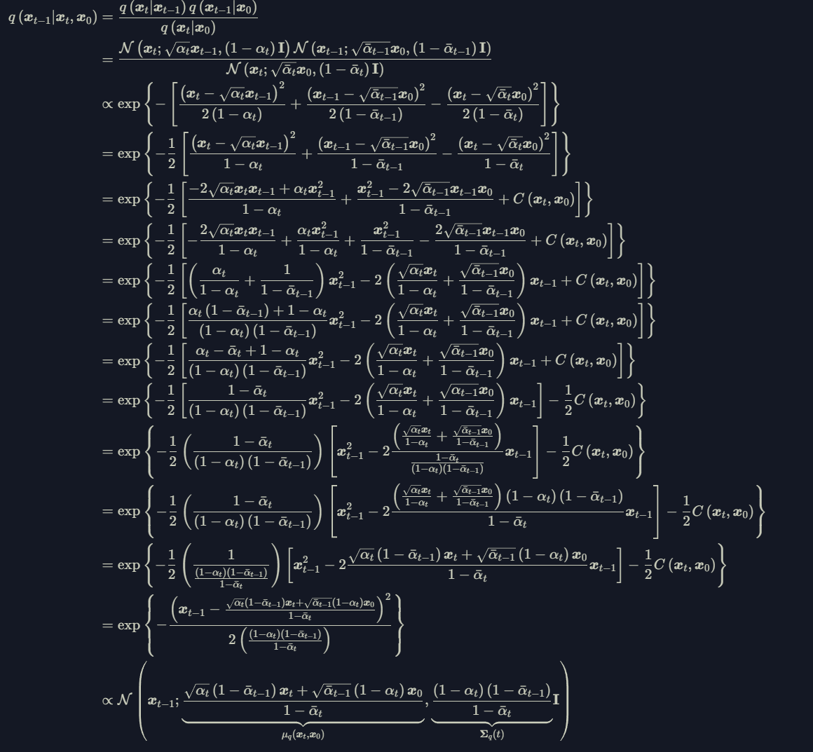
Eventually, $q(x_{t-1}|x_t,x_0)$ is expressed as follow: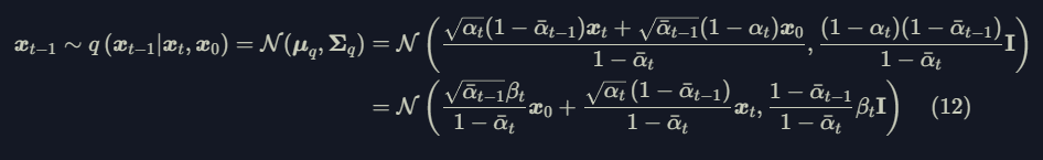
According to the theorem below:
$$
D_{\mathrm{KL}}\left(\mathcal{N}\left(\boldsymbol{x} ; \boldsymbol{\mu}_x, \boldsymbol{\Sigma}_x\right) | \mathcal{N}\left(\boldsymbol{y} ; \boldsymbol{\mu}_y, \boldsymbol{\Sigma}_y\right)\right)=\frac{1}{2}\left[\log \frac{\left|\boldsymbol{\Sigma}_y\right|}{\left|\boldsymbol{\Sigma}_x\right|}-d+\operatorname{tr}\left(\boldsymbol{\Sigma}_y^{-1} \boldsymbol{\Sigma}_x\right)+\left(\boldsymbol{\mu}_y-\boldsymbol{\mu}_x\right)^T \boldsymbol{\Sigma}_y^{-1}\left(\boldsymbol{\mu}_y-\boldsymbol{\mu}_x\right)\right]
$$
Assuming $p_\theta$ and $q$ have the same variance, then the denoising matching term can be expressed as follow:
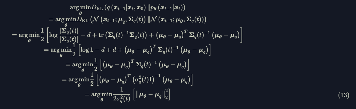
The only unknown variable in Eq.13 is $\mu_\theta$. DDPM parameterize $\mu_\theta$ using the same form of $\mu_q$ instead of directly predicting $\mu_\theta$, which gives:
$$
\mu_\theta = \frac{\sqrt{\overline\alpha_{t-1}}\beta_t}{1-\overline\alpha_t} \hat x_0 + \frac{\sqrt{\alpha_{t}}(1-\overline\alpha_{t-1})}{1-\overline\alpha_t} x_t \
= \frac{\sqrt{\overline\alpha_{t-1}}\beta_t}{1-\overline\alpha_t} \frac{x_t - \sqrt{1-\overline\alpha_t}\hat\epsilon_t}{\sqrt{\overline\alpha_t}} + \frac{\sqrt{\alpha_{t}}(1-\overline\alpha_{t-1})}{1-\overline\alpha_t} x_t \
= \frac{1}{\sqrt{\alpha_t}}x_t + \frac{1-\alpha_t}{\sqrt{1-\overline\alpha_t} \sqrt{\alpha_t}} \hat\epsilon_t (14)\
$$
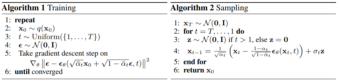
Therefore, to estimate $\mu_\theta$, we only need to predict the noise $\hat\epsilon_t=f_\theta(x_t,t)$. Eq.13 is then transformed into:
$$
\begin{aligned} & \underset{\boldsymbol{\theta}}{\arg\min} D_{\mathrm{KL}}(\left(q(x_{t-1} | x_t, x_0))\right | p_{\theta} (x_{t-1} | x_t)) = \underset{\theta}{\arg \min } \frac{1}{2 \sigma_q^2(t)} \frac{(1-\alpha_t)^2}{(1-\bar{\alpha}_t)\alpha_t}[|f_\theta (x_t, t) - \varepsilon_t |_2^2] \end{aligned} \tag{15}
$$
The final loss function $L$ can be expressed as below:
$$
L_{simple}(\theta) = E_{t, x_0, \epsilon}[|\epsilon - \epsilon_\theta(\sqrt{\overline\alpha_t}x_0 + \sqrt{1-\overline\alpha_t}\epsilon, t)|_2^2] (16)
$$
By comparing Eq.15 and Eq.16, we will find that $L$ is actually simplified, discarding the weights. As explained in DDPM, the simplified objective down-weights loss terms corresponding to small t. These terms train the network to denoise data with very small amounts of noise, so it is beneficial to down-weight them so that the network can
focus on more difficult denoising tasks at larger t terms.
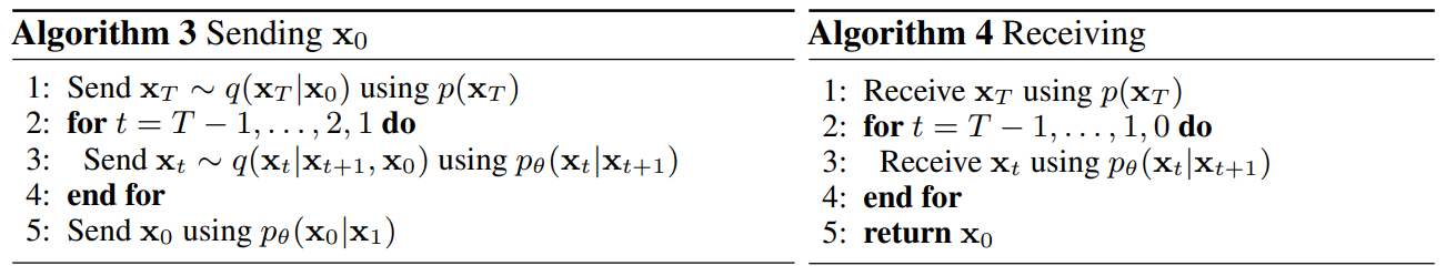
Training and Sampling
References
[1] Jonathan Ho, Ajay Jain, Pieter Abbeel; Denoising Diffusion Probabilistic Models, arXiv:2006.11239, 2020